Introduction to Forest-Guided Clustering (FGC): Simple Use Cases#
📚 This tutorial provides a basic introduction to using the Forest-Guided Clustering (FGC) Python package for interpreting trained Random Forest models. You’ll learn:
How to install the Forest-Guided Clustering package
How to apply it to your trained Random Forest model
How to interpret the resulting visualizations and insights
📦 Installation: To get started, you need to install the fgclustering package. Please follow the instructions on the official installation guide.
🚧 Note: The Forest-Guided Clustering method uncovers structure in your data by identifying the most influential features in your model’s decision-making process. However, if your Random Forest model performs poorly, the extracted feature importances may not reflect meaningful patterns in the data. Ensure that your model has reasonable predictive performance before interpreting its structure using FGC.
Imports:
[ ]:
## Import the Forest-Guided Clustering package
from fgclustering import (
    forest_guided_clustering,
    forest_guided_feature_importance,
    plot_forest_guided_clustering,
    plot_forest_guided_feature_importance,
    plot_forest_guided_decision_paths,
    DistanceRandomForestProximity,
    DistanceRandomForestLCA,
    ClusteringKMedoids,
    ClusteringClara,
)

## Imports for datasets
from palmerpenguins import load_penguins
from sklearn.datasets import load_breast_cancer, fetch_california_housing

## Additional imports for use-cases
import pandas as pd
from sklearn.ensemble import RandomForestClassifier, RandomForestRegressor
Use Case 1: Forest-Guided Clustering with a Random Forest Classifier#
In this first use case, we apply Forest-Guided Clustering to a simple binary classification problem using a Random Forest classifier. This introductory example serves as a comprehensive walkthrough of the package and its core functionality. We will demonstrate the complete Forest-Guided Clustering workflow, including cluster generation, optimization of the number of clusters, feature importance analysis, and visualization of the resulting decision patterns.
Along the way, we will introduce the main API components of the package, explain the available distance metrics and clustering strategies, discuss the most important parameters, and interpret the generated plots and outputs in detail. The goal of this section is to provide an intuitive understanding of how Forest-Guided Clustering works and how its different components can be combined to interpret Random Forest models in practice.
🎀 Data Pre-Processing and Model Training#
We use the Breast Cancer dataset from sklearn.datasets (see the official description here). This dataset consists of 569 samples, including: 212 malignant tumors (class 0) and 357 benign tumors (class 1). Each tumor is characterized by 30 numerical features, which are computed from digitized images of breast masses.
[2]:
data_breast_cancer = load_breast_cancer(as_frame=True)
data_breast_cancer = data_breast_cancer.frame
data_breast_cancer['target'] = data_breast_cancer['target'].map({0: 'malignant', 1: 'benign'})
data_breast_cancer.head()
[2]:
| mean radius | mean texture | mean perimeter | mean area | mean smoothness | mean compactness | mean concavity | mean concave points | mean symmetry | mean fractal dimension | ... | worst texture | worst perimeter | worst area | worst smoothness | worst compactness | worst concavity | worst concave points | worst symmetry | worst fractal dimension | target | |
|---|---|---|---|---|---|---|---|---|---|---|---|---|---|---|---|---|---|---|---|---|---|
| 0 | 17.99 | 10.38 | 122.80 | 1001.0 | 0.11840 | 0.27760 | 0.3001 | 0.14710 | 0.2419 | 0.07871 | ... | 17.33 | 184.60 | 2019.0 | 0.1622 | 0.6656 | 0.7119 | 0.2654 | 0.4601 | 0.11890 | malignant |
| 1 | 20.57 | 17.77 | 132.90 | 1326.0 | 0.08474 | 0.07864 | 0.0869 | 0.07017 | 0.1812 | 0.05667 | ... | 23.41 | 158.80 | 1956.0 | 0.1238 | 0.1866 | 0.2416 | 0.1860 | 0.2750 | 0.08902 | malignant |
| 2 | 19.69 | 21.25 | 130.00 | 1203.0 | 0.10960 | 0.15990 | 0.1974 | 0.12790 | 0.2069 | 0.05999 | ... | 25.53 | 152.50 | 1709.0 | 0.1444 | 0.4245 | 0.4504 | 0.2430 | 0.3613 | 0.08758 | malignant |
| 3 | 11.42 | 20.38 | 77.58 | 386.1 | 0.14250 | 0.28390 | 0.2414 | 0.10520 | 0.2597 | 0.09744 | ... | 26.50 | 98.87 | 567.7 | 0.2098 | 0.8663 | 0.6869 | 0.2575 | 0.6638 | 0.17300 | malignant |
| 4 | 20.29 | 14.34 | 135.10 | 1297.0 | 0.10030 | 0.13280 | 0.1980 | 0.10430 | 0.1809 | 0.05883 | ... | 16.67 | 152.20 | 1575.0 | 0.1374 | 0.2050 | 0.4000 | 0.1625 | 0.2364 | 0.07678 | malignant |
5 rows × 31 columns
To begin, we train a Random Forest classifier on the full Breast Cancer dataset. Instead of performing an explicit train/test split, we rely on the out-of-bag (OOB) score, which provides an internal estimate of model accuracy using the bootstrap samples generated during training. This allows us to evaluate model performance without holding out a separate test set.
[3]:
X_breast_cancer = data_breast_cancer.loc[:, data_breast_cancer.columns != 'target']
y_breast_cancer = data_breast_cancer.target

rf_breast_cancer = RandomForestClassifier(max_samples=0.8, max_depth=5, max_features='sqrt', n_estimators=100, bootstrap=True, oob_score=True, random_state=42)
rf_breast_cancer.fit(X_breast_cancer, y_breast_cancer)

print(f'OOB accuracy of prediction model: {round(rf_breast_cancer.oob_score_,3)}')
OOB accuracy of prediction model: 0.954
Compute the Forest-Guided Clusters#
Now that we have a trained Random Forest classifier, we can apply Forest-Guided Clustering (FGC) to better understand which features influence the model’s decision-making process — specifically how features contribute to distinguishing between malignant and benign tumors.
Forest-Guided Clustering is designed to interpret how a trained Random Forest model partitions and understands the data. Rather than approximating the model with surrogate explanations, FGC directly leverages the intrinsic structure of the forest, i.e. the tree traversal patterns of the samples, to derive an interpretable representation of the model’s learned decision logic.
The first step of FGC is to compute a Random-Forest-derived distance between samples. The framework currently supports two complementary distance formulations:
Proximity-based distance: Two samples are considered similar if they frequently end up in the same terminal leaf across the trees of the forest. The similarity between two samples is therefore defined by how often they share a leaf node. Samples repeatedly grouped together by the forest receive a high similarity score, whereas samples rarely sharing leaves are considered dissimilar.cThis formulation focuses on whether samples arrive at the same final decision regions of the forest.
LCA-based distance: Instead of only considering the final leaf assignment, this approach compares the entire root-to-leaf decision paths of two samples. For each tree, the similarity is determined by the depth of the deepest shared node along both paths, i.e. their Least Common Ancestor (LCA). This depth is normalized by the depth of the deeper path, so samples that share long decision-path prefixes are considered more similar, even if they eventually end up in different leaves. Unlike proximity-based distances, the LCA formulation captures how long two samples follow the same sequence of decisions before diverging, providing a more fine-grained view of the forest structure.
Both approaches transform the Random Forest into a pairwise distance matrix, which serves as the foundation for clustering. Next, a clustering algorithm is applied to this distance matrix, which can be either K-Medoids or CLARA (a scalable variant suited for larger datasets). These clustering techniques assign each sample to a cluster in a way that minimizes the average dissimilarity to the medoid (a representative sample of the cluster).
If the number of clusters (k) is not specified, FGC automatically determines the optimal number of clusters using a two-part optimization strategy:
Score: Measures the separation of target values (e.g. class labels) between clusters. A lower score indicates that clusters contain more homogeneous groups with respect to the target, reducing bias within clusters.
Jaccard Index (JI): Assesses the stability of the clustering by repeatedly subsampling the dataset and recomputing the clusters. A high JI (typically > 0.6, see here for further explanations) indicates that the clustering is consistent and robust to variation, reflecting low variance.
By balancing these two objectives, i.e. minimizing the score while maximizing stability, FGC selects clusters that are both informative and reliable.
We begin by initializing and running the clustering process using the forest_guided_clustering() function.
The function requires the following inputs:
estimator: a trained Random Forest model.X: a feature matrix containing the input data.y: the corresponding target values. The target values can be provided either as a separate vector or as a column withinX. If the target is not included in theXDataFrame, you should pass the target values directly toy, for example usingy = X["target"], and then remove the column fromXto avoid duplication.clustering_distance_metric: a Random-Forest-based distance metric defining how similarity between samples is computed from the forest structure, such asDistanceRandomForestProximity()orDistanceRandomForestLCA()clustering_strategy: determines how the forest-derived distance matrix is clustered, such asClusteringKMedoids()orClusteringClara().
Optional parameters include:
k: Number of clusters to use. This can be an integer (to use a fixed number of clusters), a tuple of two integers (to define a range over which the optimal number of clusters will be selected), or None. If None is provided (default), the optimization will run over the default range of 2 to 6 clusters.JI_bootstrap_iter: Number of bootstrap iterations for cluster stability (default: 100).JI_bootstrap_sample_size: Number of samples to use per bootstrap iteration. If set to None (default), the sample size is automatically adjusted based on the dataset size. It can also be provided as a float between 0 and 1 (indicating the fraction of the dataset to sample), or as an integer to explicitly define the number of samples.JI_discart_value: Minimum Jaccard Index threshold to consider clusters stable (default: 0.6).n_jobs: Number of parallel jobs used during bootstrapping (default: 1).random_state: Seed for reproducibility (default: 42).verbose: Whether to print progress and intermediate results (default: 1).
[4]:
fgc = forest_guided_clustering(
    k=(2,15),
    estimator=rf_breast_cancer,
    X=X_breast_cancer,
    y=y_breast_cancer,
    clustering_distance_metric=DistanceRandomForestProximity(),
    clustering_strategy=ClusteringKMedoids()
)
Using a sample size of 80.00% of the input data for Jaccard Index computation.
Using range k = (2, 15) to optimize k.
Optimizing k: 100%|██████████| 14/14 [01:27<00:00, 6.27s/it]
Optimal number of clusters k = 2

Clustering Evaluation Summary:
 k    Score  Stable  Mean_JI                                                                                                                                                Cluster_JI
 2 0.068782    True    0.998                                                                                                                                      {1: 0.999, 2: 0.998}
 3 0.074790    True    0.990                                                                                                                            {1: 0.999, 2: 0.973, 3: 0.997}
 4 0.110588    True    0.893                                                                                                                  {1: 0.929, 2: 0.701, 3: 0.952, 4: 0.991}
 5 0.119028    True    0.946                                                                                                         {1: 0.971, 2: 0.906, 3: 0.897, 4: 0.96, 5: 0.996}
 6 0.087307    True    0.874                                                                                              {1: 0.648, 2: 0.916, 3: 0.852, 4: 0.894, 5: 0.953, 6: 0.984}
 7 0.121742    True    0.855                                                                                     {1: 0.793, 2: 0.897, 3: 0.853, 4: 0.88, 5: 0.636, 6: 0.954, 7: 0.974}
 8 0.123604    True    0.895                                                                           {1: 0.873, 2: 0.951, 3: 0.796, 4: 0.896, 5: 0.905, 6: 0.791, 7: 0.97, 8: 0.975}
 9 0.112263    True    0.791                                                                {1: 0.378, 2: 0.617, 3: 0.933, 4: 0.889, 5: 0.807, 6: 0.844, 7: 0.756, 8: 0.939, 9: 0.952}
10 0.093262    True    0.745                                                      {1: 0.936, 2: 0.648, 3: 0.444, 4: 0.881, 5: 0.78, 6: 0.816, 7: 0.744, 8: 0.891, 9: 0.906, 10: 0.402}
11 0.088460    True    0.786                                           {1: 0.958, 2: 0.57, 3: 0.677, 4: 0.721, 5: 0.913, 6: 0.833, 7: 0.828, 8: 0.737, 9: 0.926, 10: 0.915, 11: 0.566}
12 0.096171    True    0.815                                 {1: 0.81, 2: 0.821, 3: 0.692, 4: 0.97, 5: 0.911, 6: 0.852, 7: 0.863, 8: 0.616, 9: 0.595, 10: 0.936, 11: 0.763, 12: 0.948}
13 0.071414    True    0.823                      {1: 0.584, 2: 0.807, 3: 0.784, 4: 0.679, 5: 0.969, 6: 0.921, 7: 0.858, 8: 0.809, 9: 0.76, 10: 0.924, 11: 0.805, 12: 0.817, 13: 0.98}
14 0.115604    True    0.853            {1: 0.974, 2: 0.85, 3: 0.829, 4: 0.769, 5: 0.921, 6: 0.785, 7: 0.831, 8: 0.773, 9: 0.587, 10: 0.85, 11: 0.938, 12: 0.96, 13: 0.995, 14: 0.883}
15 0.130065    True    0.851 {1: 0.977, 2: 0.861, 3: 0.822, 4: 0.771, 5: 0.92, 6: 0.833, 7: 0.847, 8: 0.8, 9: 0.699, 10: 0.593, 11: 0.885, 12: 0.906, 13: 0.995, 14: 0.895, 15: 0.959}
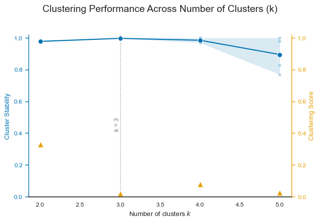
The output summarizes the optimization process used to determine the number of clusters (k) in Forest-Guided Clustering (FGC). In this example, the algorithm used 80% of the dataset in each bootstrap iteration to evaluate clustering stability and tested values of (k) ranging from 2 to 15. The optimal number of clusters was determined to be k = 2, based on the combination of a very low clustering score (0.068782) and extremely high clustering stability (Mean_JI = 0.998).
The forest_guided_clustering() function returns a Bunch object containing the following attributes:
best_k: The optimal number of clusters selected based on clustering quality and stability.ks: Array containing all evaluated values of (k).scores: Clustering quality score for each evaluated value of (k). Lower values indicate more homogeneous clusters with respect to the target variable.mean_ji: Mean Jaccard Index for each evaluated value of (k), measuring clustering stability across bootstrap iterations.stable_mask: Boolean array indicating whether each clustering solution satisfies the Jaccard stability threshold.cluster_jis: Dictionary containing the cluster-wise Jaccard Index values for every evaluated (k).cluster_labels: Dictionary mapping each evaluated value of (k) to the corresponding cluster assignments of all samples.model_type: Indicates whether the fitted Random Forest model is a classifier or regressor.
To further interpret the optimization process, FGC provides the plot_forest_guided_clustering() function, which visualizes clustering quality and stability across all evaluated values of (k).
The resulting plot combines:
the clustering score, measuring how well the clusters separate the target variable,
the mean Jaccard Index (JI), measuring overall clustering stability,
and the cluster-wise Jaccard Indices, showing the stability of each individual cluster.
[5]:
plot_forest_guided_clustering(
    ks=fgc.ks,
    scores=fgc.scores,
    mean_ji=fgc.mean_ji,
    cluster_jis=fgc.cluster_jis,
    best_k=fgc.best_k,
    JI_discart_value=0.6
)
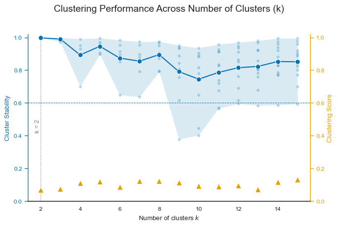
This visualization is particularly useful because it allows users to investigate alternative clustering solutions beyond the automatically selected best_k. In many real-world datasets, multiple values of (k) may produce similarly good scores and stability values. In such cases, choosing a smaller number of clusters may lead to a more interpretable and easier-to-communicate grouping structure, whereas larger values of (k) may reveal more fine-grained subpopulations that can be useful for
exploratory analyses.
For our use case, the plot shows that k = 2 provides the most stable overall clustering solution, with an almost perfect mean Jaccard Index close to 1.0 while also achieving one of the lowest clustering scores. As (k) increases, cluster stability gradually decreases and individual clusters become more heterogeneous in their robustness. Although some larger values of (k) still achieve competitive scores, they introduce increasingly unstable subclusters, suggesting that the underlying data
structure is most naturally separated into two major groups. At the same time, intermediate values such as k = 3 or k = 5 may still provide biologically meaningful subgroup structures if a more detailed interpretation is desired.
Evaluate Feature Importance#
Now that we have the optimal clustering of data points guided by the Random Forest decision paths, we can calculate which features are most distinctive of the different clusters. The forest_guided_feature_importance() function quantifies how important each feature is for differentiating between the discovered clusters. It does so without relying on surrogate models, and instead directly compares feature distributions:
Local Feature Importance is computed by comparing the feature distribution within each cluster to the overall feature distribution in the dataset.
Global Feature Importance is the average of these distances across all clusters, highlighting features that consistently differentiate between clusters.
To quantify these differences, the function supports two distance metrics:
Wasserstein Distance: suited for mostly continuous features
Jensen-Shannon Distance: suited for mostly categorical or binary features
These distances capture the dissimilarity between distributions, i.e., how much the feature’s distribution changes from cluster to cluster, relative to the global distribution.
The forest_guided_feature_importance() function computes how strongly individual features contribute to the separation between clusters.
The function requires the following inputs:
X: the feature matrix used for computing feature importance. While this matrix must contain the same samples that were used during clustering, it may contain a different set of features than those used to train the Random Forest model. This is possible because the clustering itself depends only on the sample-level similarity structure derived from the Random Forest, rather than directly on the feature space used during training.y: the target variable.cluster_labels: the cluster assignments produced byforest_guided_clustering().
Optional parameters include:
y_pred: Optional predicted target values aligned with the samples inX. When provided, these predictions are included in the returned clustering table and downstream visualizations, enabling direct comparison between observed and predicted target values within clusters.feature_importance_distance_metric: Distance metric used to compare cluster-specific feature distributions against the background distribution. Supported options are"wasserstein"and"jensenshannon"(default:"wasserstein").verbose: Verbosity level controlling progress output during feature importance computation (default:1).
[6]:
feature_importance = forest_guided_feature_importance(
    X=X_breast_cancer,
    y=y_breast_cancer,
    y_pred=rf_breast_cancer.predict(X_breast_cancer),
    cluster_labels=fgc.cluster_labels[fgc.best_k],
)
100%|██████████| 30/30 [00:00<00:00, 2250.57it/s]
The function returns a Bunch object containing the following outputs:
feature_importance_local: A DataFrame containing the cluster-specific feature importance values. Each row corresponds to a feature and each column corresponds to a cluster. The values quantify how strongly the feature distribution within a cluster differs from the background distribution across the full dataset. Higher values indicate that the feature contributes more strongly to distinguishing that cluster from the remaining samples.feature_importance_global: A Series containing the global feature importance values obtained by averaging the local feature importance scores across all clusters. This provides an overall ranking of the features that most strongly explain the clustering structure learned from the Random Forest model.data_clustering: A clustering table containing the original feature values, the target values (target), optionally the predicted target values (predicted_target) ify_predwas provided, and the assigned cluster labels (cluster). The feature columns are automatically sorted according to their global feature importance, facilitating downstream visualization and interpretation of the cluster-specific decision patterns.
Visualize the Results#
Once the local and global feature importances have been computed, the results can be visualized using the plot_forest_guided_feature_importance() function. This visualization highlights which features contribute most strongly to separating the identified clusters, both globally across all clusters and locally within each individual cluster.
The function requires the following inputs:
feature_importance_local: A DataFrame containing cluster-specific (local) feature importance values.feature_importance_global: A Series containing global feature importance values.
Optional parameters include:
top_n: Number of top-ranked features to include in the visualization. IfNone, all features are shown.num_cols: Maximum number of subplot columns in the figure layout (default:4).reorder: IfTrue, local feature importance panels are reordered according to the global feature ranking, making it easier to directly compare clusters using a shared feature order (default:False).recolor: IfTrue, local feature bars are colored according to the global feature ranking, improving visual consistency between the global and local importance panels (default:False).color_spec: Optional dictionary used to override entries of the default plotting color specification.show: IfTrue(default), the figure is displayed immediately. IfFalse, the Matplotlib figure and axes objects are returned, allowing further customization before rendering.save: Optional output path used to save the generated figure. IfNone, the figure is not written to disk.
[7]:
plot_forest_guided_feature_importance(
    feature_importance_local=feature_importance.feature_importance_local,
    feature_importance_global=feature_importance.feature_importance_global,
)

The resulting plot helps interpret which features are most responsible for the forest-defined segmentation of the data. In the example above, we can see that approximately half of the features contribute to distinguishing clusters.
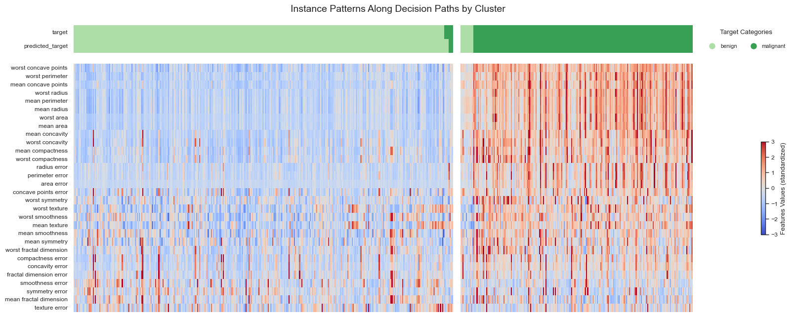
Now that we have clustered the data using Random Forest decision paths and identified the most important features, we can visually explore how the forest partitions the data using the plot_forest_guided_decision_paths() function. This visualization provides deeper insight into the learned decision structure of the Random Forest model by combining complementary global and cluster-level visualizations.
The function can generate up to three different visualization types:
Heatmap: A cluster-level overview showing feature enrichment/depletion patterns together with the target value distribution across clusters. This visualization helps identify which clusters correspond to which classes or target ranges. Samples appearing in unexpected clusters may indicate outliers, mislabeled observations, or biologically distinct subgroups.
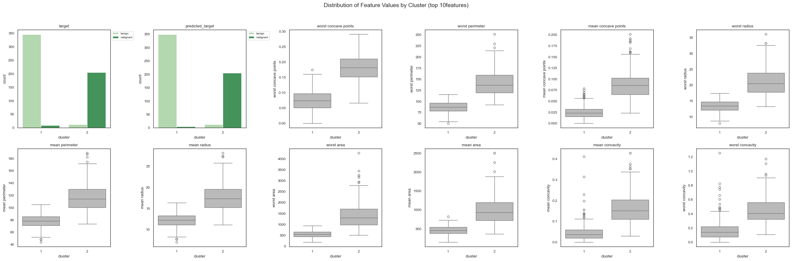
Feature Distributions: Distribution plots showing the raw feature values across clusters without standardization. These plots help inspect within-cluster variance, overlaps between clusters, and the actual feature value ranges contributing to the separation.
Dot Plot: A compact summary visualization combining local and global feature importance information. The dot plot provides an efficient overview of which features drive each cluster and in which direction they deviate from the background distribution. Compared to displaying many individual distribution plots, the dot plot offers a substantially more compact and interpretable representation of the cluster-specific decision structure.
The function requires the following inputs:
data_clustering: A DataFrame containing the cluster labels, target values, optional predicted target values, and ranked feature columns returned byforest_guided_feature_importance().feature_importance_global: Global feature importance values used for feature ranking and selection.feature_importance_local: Cluster-specific feature importance values used for the dot plot visualization.model_type: Indicates whether the fitted model is a classifier or regressor, returned byforest_guided_clustering().
Optional parameters include:
draw_distributions: Whether to generate feature distribution plots for each cluster (default:True).draw_dotplot: Whether to generate the compact feature-importance dot plot (default:True).draw_heatmap: Whether to generate the cluster heatmap visualization (default:True).heatmap_type: Heatmap rendering mode, either"static"(default) or"interactive".top_n: Number of top-ranked features to visualize based on global feature importance. IfNone, all features are included.num_cols: Number of subplot columns used for the distribution plot layout (default:6).color_spec: Optional dictionary overriding entries of the default plotting color specification.show: IfTrue(default), the generated figures are displayed immediately. IfFalse, the plot objects are returned for further customization.save: Optional output path used to save the generated figures. IfNone, the figures are not written to disk.
[8]:
plot_forest_guided_decision_paths(
    data_clustering=feature_importance.data_clustering,
    feature_importance_global=feature_importance.feature_importance_global,
    feature_importance_local=feature_importance.feature_importance_local,
    model_type=fgc.model_type,
    draw_heatmap=True,
    draw_distributions=False,
    draw_dotplot=False,
)
[9]:
plot_forest_guided_decision_paths(
    data_clustering=feature_importance.data_clustering,
    feature_importance_global=feature_importance.feature_importance_global,
    feature_importance_local=feature_importance.feature_importance_local,
    model_type=fgc.model_type,
    draw_heatmap=False,
    draw_distributions=True,
    draw_dotplot=False,
    top_n=10,
)
[10]:
plot_forest_guided_decision_paths(
    data_clustering=feature_importance.data_clustering,
    feature_importance_global=feature_importance.feature_importance_global,
    feature_importance_local=feature_importance.feature_importance_local,
    model_type=fgc.model_type,
    draw_heatmap=False,
    draw_distributions=False,
    draw_dotplot=True,
)
From the resulting visualizations, we can draw several important conclusions about how the Random Forest model separates malignant and benign tumors:
The two target classes are almost perfectly separated into two distinct clusters. Both the heatmap and the target distribution plots show that only a very small number of samples are assigned to the “opposite” cluster. These samples may represent biologically ambiguous cases, mislabeled observations, noisy measurements, or potential outliers that warrant further investigation.
The globally most important features identified by Forest-Guided Clustering are highly consistent across all visualization modalities. Features such as worst concave points, worst perimeter, mean concave points, worst radius, and mean perimeter consistently appear among the strongest cluster-separating variables in the heatmap, distribution plots, and dot plot.
The feature distribution plots show that samples belonging to the malignant cluster generally exhibit substantially larger feature values than samples in the benign cluster. In particular, malignant tumors tend to have larger radii and perimeters, higher concavity and compactness, and more pronounced concave points. These characteristics are consistent with more irregular and invasive tumor morphologies.
The dot plot provides a compact summary of these cluster-specific feature patterns. Larger dots indicate features with stronger importance for distinguishing the clusters, while the color encodes the direction of the effect relative to the global background distribution. This makes it possible to rapidly identify which features are most characteristic for each cluster without inspecting dozens of individual distribution plots.
Use Case 2: Forest-Guided Clustering for a Random Forest Classifier with Categorical Features#
The second use case demonstrates how Forest-Guided Clustering (FGC) can be applied to interpret a multiclass Random Forest classification model, which contains a mixture of continuous and categorical features.
The primary goal of this example is to illustrate how FGC naturally supports the interpretation of categorical variables. Importantly, Forest-Guided Clustering operates on sample-level similarities derived from the Random Forest model rather than directly on the original feature representation used during model training. As a result, the feature space used for downstream FGC analysis does not need to exactly match the feature representation used by the classifier itself.
This becomes particularly useful for categorical variables. During Random Forest training, categorical features are often transformed using one-hot encoding because scikit-learn estimators require numerical input representations. However, for Forest-Guided Clustering analysis and visualization, we can instead provide the original human-readable categorical features directly. Since clustering is performed on the learned sample relationships rather than on the raw feature vectors, FGC can correctly analyze and visualize the original categorical variables without requiring the one-hot encoded representation.
This enables substantially more interpretable downstream analyses, especially for heatmaps, feature importance visualizations, and distribution plots, where original categorical labels are much easier to interpret than sparse one-hot encoded columns.
🐧 Data Pre-Processing and Model Training#
Here, we train a Random Forest classifier on the Palmer Penguins dataset from the palmerpenguins package. For more information about this dataset, see the Palmer Penguins GitHub repository. The dataset includes 344 penguin observations collected from islands in the Palmer Archipelago near Palmer Station, Antarctica. It contains three species of penguins: 146 Adelie, 68 Chinstrap, and 119 Gentoo. Each penguin is described by a combination of
numerical and categorical features, including body size measurements, clutch observations, blood isotope ratios, and sex.
[11]:
data_penguins = load_penguins()

# Remove the instances with missing values and check how many we are left with
print(f"Before omiting the missing values the dataset has {data_penguins.shape[0]} instances")
data_penguins.dropna(inplace=True)
print(f"After omiting the missing values the dataset has {data_penguins.shape[0]} instances")

data_penguins.head()
Before omiting the missing values the dataset has 344 instances
After omiting the missing values the dataset has 333 instances
[11]:
| species | island | bill_length_mm | bill_depth_mm | flipper_length_mm | body_mass_g | sex | year | |
|---|---|---|---|---|---|---|---|---|
| 0 | Adelie | Torgersen | 39.1 | 18.7 | 181.0 | 3750.0 | male | 2007 |
| 1 | Adelie | Torgersen | 39.5 | 17.4 | 186.0 | 3800.0 | female | 2007 |
| 2 | Adelie | Torgersen | 40.3 | 18.0 | 195.0 | 3250.0 | female | 2007 |
| 4 | Adelie | Torgersen | 36.7 | 19.3 | 193.0 | 3450.0 | female | 2007 |
| 5 | Adelie | Torgersen | 39.3 | 20.6 | 190.0 | 3650.0 | male | 2007 |
We trained a Random Forest classifier on the penguins dataset. To keep the process simple and because Random Forests provide an out-of-bag (OOB) accuracy estimate, we did not perform a separate train/test split. Additionally, to incorporate categorical features into the model, we applied one-hot encoding using dummy variables, making them suitable for use with the Random Forest classifier.
[12]:
# preprocess categorical features such that they can be used for the RF model
data_penguins_encoded = pd.get_dummies(data_penguins, columns=['island', 'sex'], prefix=['island', 'sex'], drop_first=True)

X_penguins = data_penguins_encoded.loc[:, data_penguins_encoded.columns != 'species']
y_penguins = data_penguins_encoded.species

rf_penguins = RandomForestClassifier(max_samples=0.8, max_depth=5, max_features='sqrt', n_estimators=100, bootstrap=True, oob_score=True, random_state=42)
rf_penguins.fit(X_penguins, y_penguins)

print(f'OOB accuracy of prediction model: {round(rf_penguins.oob_score_,3)}')
OOB accuracy of prediction model: 0.985
Compute the Forest-Guided Clusters#
We now apply the Forest-Guided Clustering (FGC) method to gain insight into which characteristics most strongly influence the classification of the different penguin species. To do this, we use the preprocessed penguins dataset along with the trained Random Forest classifier as input to the forest_guided_clustering() function. This function requires the trained estimator, the feature matrix X, the corresponding target labels y, a distance metric (here we use
DistanceRandomForestProximity()), and a clustering strategy such as ClusteringKMedoids().
Once initialized, the clustering process is executed and returns the optimal number of clusters along with cluster assignments for each sample. For more details on the function parameters, please refer to the binary classification example above.
[13]:
fgc = forest_guided_clustering(
    k=(2,5),
    estimator=rf_penguins,
    X=X_penguins,
    y=y_penguins,
    clustering_distance_metric=DistanceRandomForestProximity(),
    clustering_strategy=ClusteringKMedoids(method="fasterpam", max_iter=200)
)
Using a sample size of 80.00% of the input data for Jaccard Index computation.
Using range k = (2, 5) to optimize k.
Optimizing k: 100%|██████████| 4/4 [00:21<00:00, 5.27s/it]
Optimal number of clusters k = 3

Clustering Evaluation Summary:
 k    Score  Stable  Mean_JI                                       Cluster_JI
 2 0.329337    True    0.978                             {1: 0.981, 2: 0.974}
 3 0.018666    True    0.997                   {1: 0.996, 2: 0.997, 3: 0.997}
 4 0.077212    True    0.985             {1: 1.0, 2: 0.969, 3: 0.973, 4: 1.0}
 5 0.025349    True    0.895 {1: 0.899, 2: 0.979, 3: 0.827, 4: 0.769, 5: 1.0}
[14]:
plot_forest_guided_clustering(
    ks=fgc.ks,
    scores=fgc.scores,
    mean_ji=fgc.mean_ji,
    cluster_jis=fgc.cluster_jis,
    best_k=fgc.best_k,
)
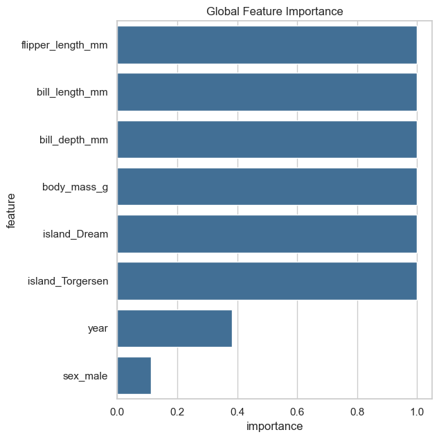
Evaluate Feature Importance#
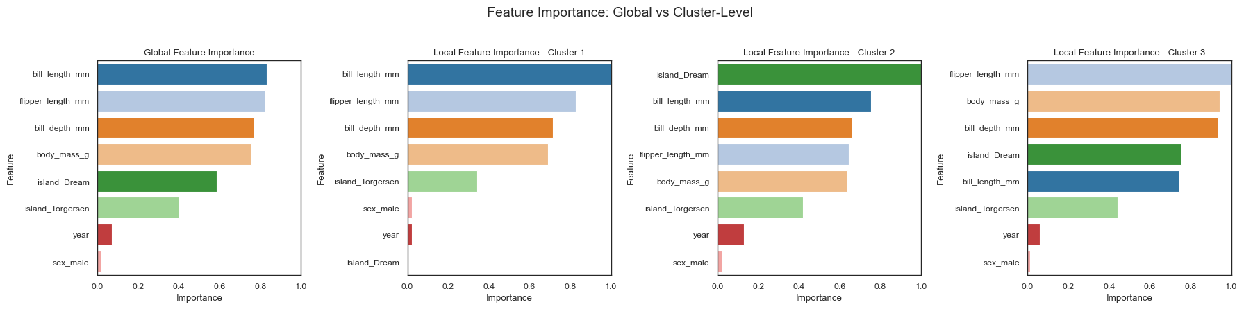
Based on the output of the forest_guided_clustering() function, we observe that the optimal number of clusters is k = 3, which yields the lowest clustering score while maintaining high stability, as indicated by a strong Jaccard Index. This aligns well with the true number of penguin species in the dataset and reflects the model’s ability to distinguish meaningful subgroups. When examining the feature importance, we notice that categorical variables such as island have been one-hot
encoded, resulting in multiple binary features (e.g., island_Dream, island_Torgersen). Each represents a category, making interpretation more difficult.
[15]:
feature_importance = forest_guided_feature_importance(
    X=X_penguins,
    y=y_penguins,
    y_pred=rf_penguins.predict(X_penguins),
    cluster_labels=fgc.cluster_labels[fgc.best_k],
    feature_importance_distance_metric="jensenshannon",
)

plot_forest_guided_feature_importance(
    feature_importance_local=feature_importance.feature_importance_local,
    feature_importance_global=feature_importance.feature_importance_global,
    recolor=True,
)
100%|██████████| 8/8 [00:00<00:00, 697.41it/s]
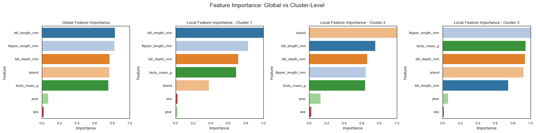
To improve interpretability, we can provide an alternative feature matrix when computing feature importance. This alternative matrix should contain the original, unencoded categorical variables and must preserve the same number and order of samples as the matrix used during forest guided clustering, as the clustering is based on sample proximities, not feature values. You can pass this alternative matrix to the forest_guided_feature_importance() function to ensure the calculated distances
and importance scores reflect the original categorical structure. This makes the output plots more intuitive and interpretable for both local and global feature importance, as well as for the decision path visualizations.
[16]:
X_add_features = data_penguins.drop('species', axis=1)
X_add_features['island'] = X_add_features['island'].astype('category')
X_add_features['sex'] = X_add_features['sex'].astype('category')

feature_importance = forest_guided_feature_importance(
    X=X_add_features,
    y=y_penguins,
    y_pred=rf_penguins.predict(X_penguins),
    cluster_labels=fgc.cluster_labels[fgc.best_k],
    feature_importance_distance_metric="jensenshannon",
)

plot_forest_guided_feature_importance(
    feature_importance_local=feature_importance.feature_importance_local,
    feature_importance_global=feature_importance.feature_importance_global,
    recolor=True,
)
100%|██████████| 7/7 [00:00<00:00, 579.80it/s]
Visualize the Results#
[17]:
plot_forest_guided_decision_paths(
    data_clustering=feature_importance.data_clustering,
    feature_importance_global=feature_importance.feature_importance_global,
    feature_importance_local=feature_importance.feature_importance_local,
    model_type=fgc.model_type,
    num_cols=5,
    draw_heatmap=True,
    draw_distributions=True,
    draw_dotplot=False,
    color_spec={
            "color_target_cat": "deep",
            "color_features_cat": "Blues",
        }
)
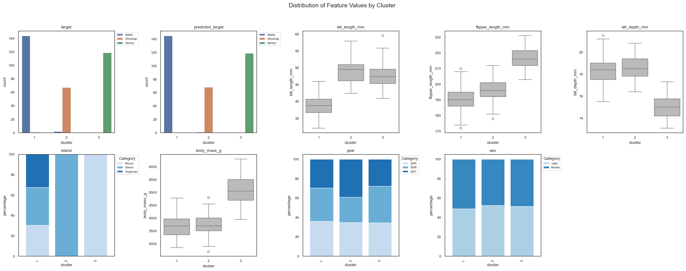
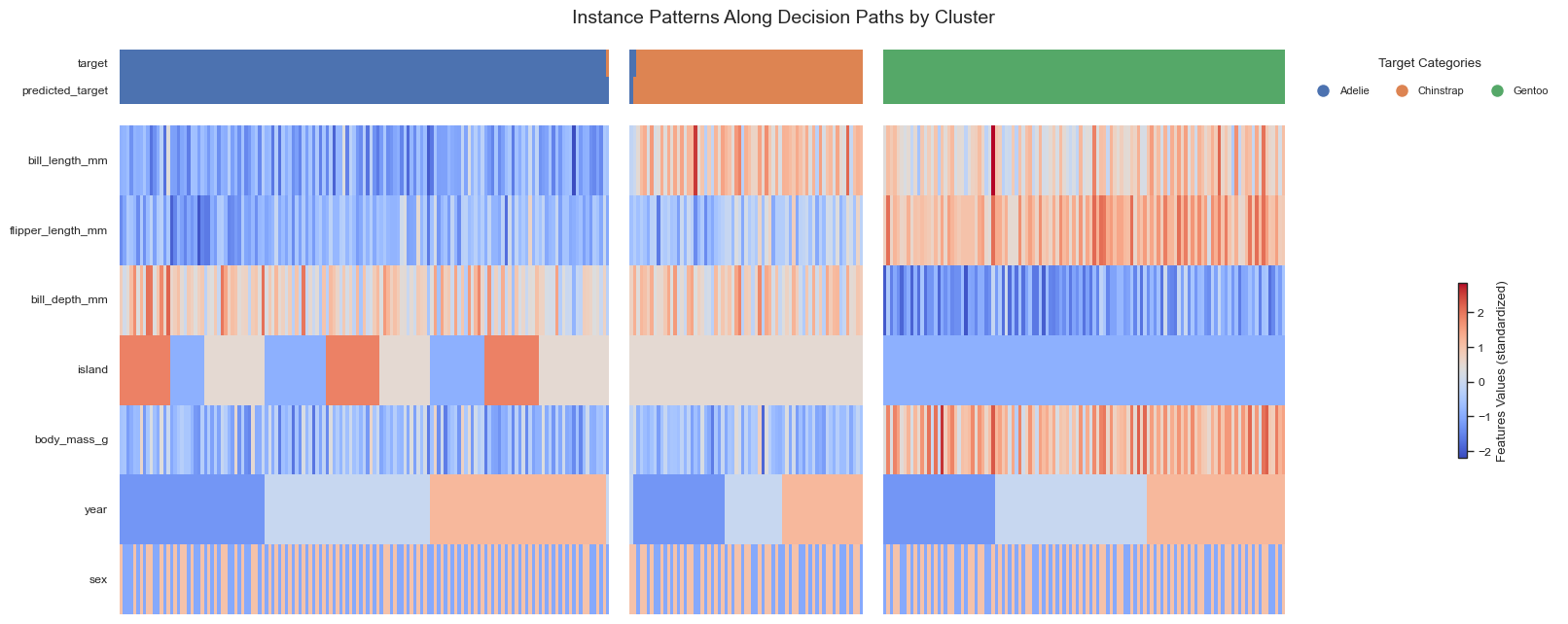
From the resulting plots, we can draw several important conclusions regarding the clustering and its alignment with the true penguin species:
The three penguin species are almost perfectly separated into the three discovered clusters. Only a small number of Adelie penguins are misassigned, which may warrant further inspection, e.g. to check for measurement anomalies or natural variability.
All features, with the exception of year and sex, contribute significantly to distinguishing the clusters, as evidenced by their global and local feature importance values and their differentiated distributions across clusters.
Cluster 0 contains exclusively Adelie penguins. These penguins are distributed across all three islands and are characterized by short flipper and bill lengths, low body mass, and deep bills.
Cluster 1 predominantly contains Chinstrap penguins. These birds are defined by relatively short flipper length and body mass, but long and deep bills. Interestingly, they are found only on Biscoe Island.
Cluster 2 consists solely of Gentoo penguins. This species exhibits opposing traits compared to Adelie penguins, such as longer flipper and bill lengths, higher body mass, and shallower bills. Gentoo penguins are exclusively observed on Dream Island.
These results illustrate how Forest-Guided Clustering captures biologically meaningful structure in the data, aligning well with known species distinctions and offering a useful interpretation of the Random Forest’s decision patterns.
Use Case 3: Forest-Guided Clustering for Regression Models#
This use case demonstrates how Forest-Guided Clustering (FGC) can be applied to interpret a Random Forest Regressor on a large-scale regression dataset. In contrast to the previous classification examples, regression forests typically learn substantially deeper and more fine-grained decision structures because they recursively partition a continuous target space into increasingly homogeneous regions.
A key focus of this example is therefore the use of the LCA-based distance metric (DistanceRandomForestLCA()), which is particularly well suited for deep regression forests. Classical proximity-based distances rely on samples ending up in the same terminal leaf. However, in large regression forests, samples often terminate in unique leaves, resulting in extremely sparse proximity matrices with limited structural information.
The LCA-based distance metric addresses this limitation by comparing the shared decision-path structure between samples instead of only their final leaf assignments. Two samples are considered similar if they follow the same sequence of decisions for a large fraction of the tree depth, even if they eventually diverge into different terminal nodes. This produces a denser and more informative similarity representation for fine-grained regression models.
This example additionally demonstrates how FGC can be scaled to larger datasets using the CLARA clustering strategy (ClusteringClara()), which performs efficient medoid-based clustering on repeated subsamples instead of requiring full clustering on the entire dataset, and the memory-efficient distance matrix implementation (memory_efficient=True), which stores temporary pairwise distance matrices as disk-backed memory-mapped arrays rather than fully allocating them in RAM.
Together, these components enable Forest-Guided Clustering to remain computationally practical even for large datasets and complex regression forests while still providing interpretable cluster structures and feature-level explanations of the model’s learned decision patterns.
🏘️ Data Pre-Processing and Model Training#
We use the California Housing dataset from sklearn.datasets (dataset details here), which includes 20,640 observations of median house values in California districts (expressed in $100,000) described by 8 numerical features, such as median income, housing age, and geographic coordinates.
[ ]:
data_housing = fetch_california_housing(as_frame=True).frame
data_housing.head()
| MedInc | HouseAge | AveRooms | AveBedrms | Population | AveOccup | Latitude | Longitude | MedHouseVal | |
|---|---|---|---|---|---|---|---|---|---|
| 0 | 8.3252 | 41.0 | 6.984127 | 1.023810 | 322.0 | 2.555556 | 37.88 | -122.23 | 4.526 |
| 1 | 8.3014 | 21.0 | 6.238137 | 0.971880 | 2401.0 | 2.109842 | 37.86 | -122.22 | 3.585 |
| 2 | 7.2574 | 52.0 | 8.288136 | 1.073446 | 496.0 | 2.802260 | 37.85 | -122.24 | 3.521 |
| 3 | 5.6431 | 52.0 | 5.817352 | 1.073059 | 558.0 | 2.547945 | 37.85 | -122.25 | 3.413 |
| 4 | 3.8462 | 52.0 | 6.281853 | 1.081081 | 565.0 | 2.181467 | 37.85 | -122.25 | 3.422 |
We trained a Random Forest Regressor on the California Housing dataset. Since the model provides out-of-bag (OOB) scores, we skipped creating separate train/test splits for simplicity.
[19]:
X_housing = data_housing.loc[:, data_housing.columns != 'MedHouseVal']
y_housing = data_housing.MedHouseVal

rf_housing = RandomForestRegressor(max_samples=0.8, max_depth=20, max_features='log2', n_estimators=100, bootstrap=True, oob_score=True, random_state=42)
rf_housing.fit(X_housing, y_housing)

print(f'OOB accuracy of prediction model: {round(rf_housing.oob_score_,3)}')
OOB accuracy of prediction model: 0.819
Forest-Guided Clustering Results#
We apply forest_guided_clustering() using the LCA-based distance metric (DistanceRandomForestLCA()) together with the scalable ClusteringClara() strategy.
For regression forests, we prefer the LCA-based distance over the classical proximity-based distance because deep regression trees often produce sparse proximity matrices where samples rarely share terminal leaves. The LCA formulation instead compares shared decision-path structure, yielding a denser and more informative similarity representation.
To handle the larger California housing dataset efficiently, we additionally enable memory_efficient=True, which stores temporary distance matrices as disk-backed memory-mapped arrays instead of fully allocating them in RAM.
[20]:
fgc = forest_guided_clustering(
    k=(2,5),
    estimator=rf_housing,
    X=X_housing,
    y=y_housing,
    clustering_distance_metric=DistanceRandomForestLCA(memory_efficient=True, dir_distance_matrix="./"),
    clustering_strategy=ClusteringClara(sampling_iter=5, sub_sample_size=0.6, method="fasterpam"),
    JI_bootstrap_iter=5,
    JI_bootstrap_sample_size=0.7,
    n_jobs=4,
)
Using range k = (2, 5) to optimize k.
Optimizing k: 100%|██████████| 4/4 [24:13<00:00, 363.36s/it]
Optimal number of clusters k = 5

Clustering Evaluation Summary:
 k    Score  Stable  Mean_JI                                         Cluster_JI
 2 0.961174    True    0.928                               {1: 0.925, 2: 0.931}
 3 0.601106    True    0.940                     {1: 0.916, 2: 0.921, 3: 0.983}
 4 0.582561    True    0.810           {1: 0.736, 2: 0.693, 3: 0.866, 4: 0.947}
 5 0.539363    True    0.905 {1: 0.943, 2: 0.889, 3: 0.892, 4: 0.918, 5: 0.882}
[23]:
feature_importance = forest_guided_feature_importance(
    X=X_housing,
    y=y_housing,
    cluster_labels=fgc.cluster_labels[fgc.best_k],
    feature_importance_distance_metric="wasserstein",
)
plot_forest_guided_feature_importance(
    feature_importance_local=feature_importance.feature_importance_local,
    feature_importance_global=feature_importance.feature_importance_global,
    reorder=True,
)
100%|██████████| 8/8 [00:00<00:00, 37.74it/s]
[24]:
plot_forest_guided_decision_paths(
    data_clustering=feature_importance.data_clustering,
    feature_importance_global=feature_importance.feature_importance_global,
    feature_importance_local=feature_importance.feature_importance_local,
    model_type=fgc.model_type,
    num_cols=5,
    draw_heatmap=False,
    draw_distributions=True,
    draw_dotplot=True,
)
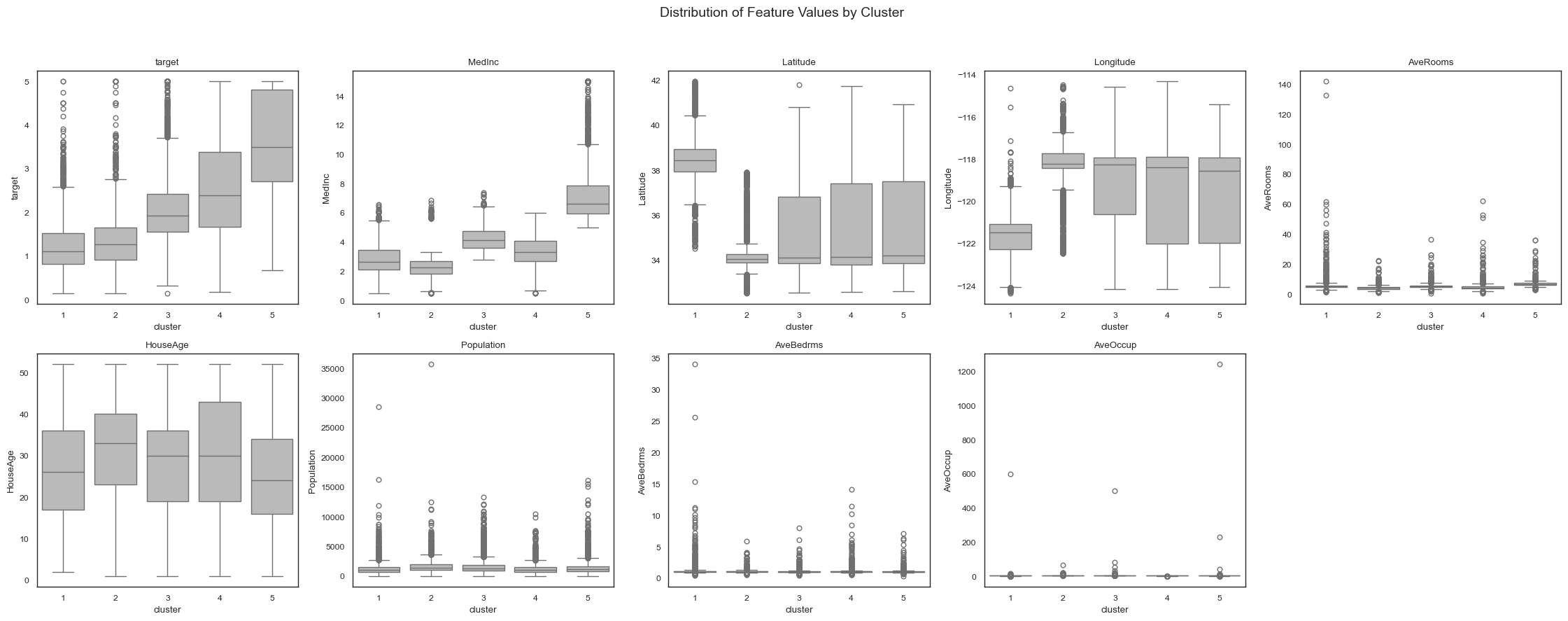
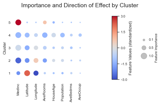
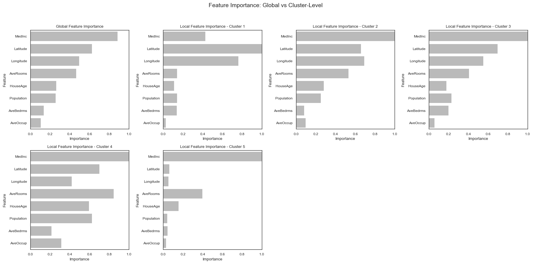
The clustering results reveal five distinct subgroups within the California housing dataset, each corresponding to different socioeconomic and geographic housing patterns.
Clusters 1 and 2 correspond to lower-valued housing regions. Both clusters exhibit low median income and relatively small homes, but they differ strongly in geographic location:
Cluster 1 is associated with higher latitudes and more eastern longitudes, suggesting inland regions with lower housing prices.
Cluster 2 is concentrated around lower latitudes and more coastal longitudes, indicating lower-income coastal urban areas.
Clusters 3 and 4 capture intermediate housing markets:
Cluster 3 contains medium-income neighborhoods with moderately larger homes and broader geographic spread.
Cluster 4 is characterized by relatively large homes and higher house age, suggesting established suburban or residential regions with stable housing values.
Cluster 5 represents the highest-valued housing regions. This cluster is characterized by very high median income (
MedInc), large homes with many rooms, and relatively low occupancy. These areas likely correspond to affluent residential neighborhoods with expensive housing markets.
Across all clusters, median income (``MedInc``) emerges as the dominant feature driving the clustering structure, followed by geographic location (Latitude, Longitude) and housing size indicators such as AveRooms. The feature importance plots show that different clusters are defined not only by different income levels, but also by distinct combinations of spatial and structural housing characteristics.
The visualizations further highlight the strongly nonlinear relationship between geographic location and housing value. Latitude and longitude contribute differently across clusters, indicating that the influence of location on housing prices depends heavily on regional context rather than following a simple linear trend. This illustrates why nonlinear models such as Random Forests are particularly effective for this dataset.
Overall, Forest-Guided Clustering reveals meaningful and interpretable subpopulations within the regression problem, ranging from lower-income inland housing regions to affluent high-value residential areas. By grouping samples according to shared Random Forest decision structures, FGC provides insight into how the model internally partitions complex socioeconomic and geographic patterns in the data.