Special Case: Inference with Forest-Guided Clustering#
📚 In this tutorial, we explore how Forest-Guided Clustering (FGC) can be extended beyond training data to draw meaningful inferences on unseen test data. Typically, when training a Random Forest model, we split our dataset into a training and test set to assess the model’s generalization performance usually through metrics like accuracy or R². However, performance metrics alone don’t tell the full story. They quantify how well the model predicts, but not how well its learned structure and explanations transfer to new data. FGC goes a step further: by analyzing the decision structure of the Random Forest, it enables us to check whether the patterns discovered during training also hold for the test set. This allows us to not only test the predictive power of our model, but also its interpretability power.
📦 Installation: To get started, you need to install the fgclustering package. Please follow the instructions on the official installation guide.
🚧 Note: For a general introduction to FGC, please refer to our Introduction Notebook.
Imports:
[ ]:
## Import the Forest-Guided Clustering package
from fgclustering import (
    forest_guided_clustering,
    forest_guided_feature_importance,
    plot_forest_guided_decision_paths,
    DistanceRandomForestLCA,
    ClusteringKMedoids,
)

## Imports for datasets
from sklearn.datasets import fetch_california_housing

## Additional imports for use-cases
from sklearn.ensemble import RandomForestRegressor
🏠 The California Housing Dataset#
To demonstrate how Forest-Guided Clustering (FGC) can be applied at inference time, we will again use the California Housing dataset (see Use Case 3 for a detailed description). For this example, we will use the first 1,000 samples as our training set, on which we train a Random Forest Regressor.
[2]:
data_housing = fetch_california_housing(as_frame=True).frame

data_housing_train = data_housing.iloc[:1000]
X_housing_train = data_housing_train.loc[:, data_housing_train.columns != 'MedHouseVal']
y_housing_train = data_housing_train.MedHouseVal

rf_housing = RandomForestRegressor(max_samples=0.8, max_depth=20, max_features='log2', n_estimators=100, bootstrap=True, oob_score=True, random_state=42)
rf_housing.fit(X_housing_train, y_housing_train)

print(f'Train Set R^2 of prediction model: {round(rf_housing.score(X_housing_train, y_housing_train),3)}')
Train Set R^2 of prediction model: 0.956
🔍 Interpreting Test Set Behavior with Forest-Guided Clustering#
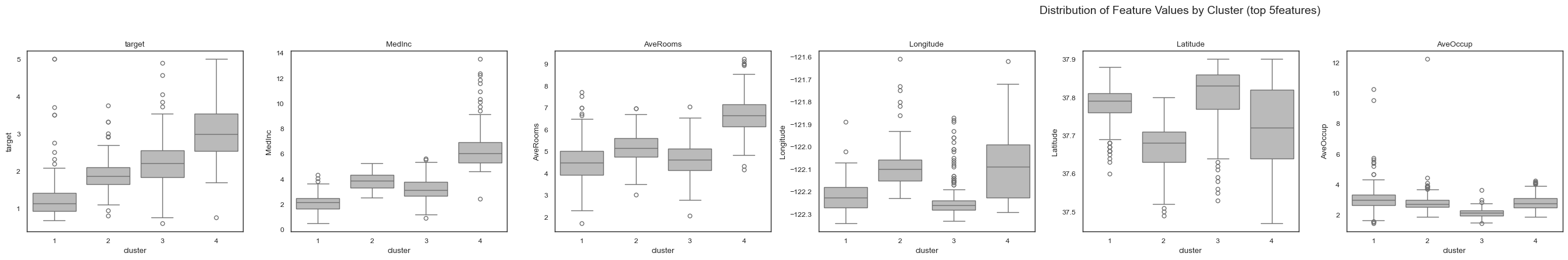
To understand the relationship between housing values and the input features (e.g. median income, house age, etc.), we start by applying the Forest-Guided Clustering (FGC) method on the training dataset using the trained Random Forest Regressor.
[3]:
fgc = forest_guided_clustering(
    estimator=rf_housing,
    X=data_housing_train,
    y='MedHouseVal',
    clustering_distance_metric=DistanceRandomForestLCA(),
    clustering_strategy=ClusteringKMedoids(method="fasterpam"),
    JI_discart_value=0.9
)
Using a sample size of 80.00% of the input data for Jaccard Index computation.
Using range k = (2, 6) to optimize k.
Optimizing k: 100%|██████████| 5/5 [00:49<00:00, 9.87s/it]
Optimal number of clusters k = 4

Clustering Evaluation Summary:
 k    Score  Stable  Mean_JI                                                  Cluster_JI
 2 0.849413   False    0.804                                         {1: 0.748, 2: 0.86}
 3 0.469388    True    0.958                              {1: 0.952, 2: 0.957, 3: 0.966}
 4 0.432164    True    0.960                    {1: 0.975, 2: 0.955, 3: 0.937, 4: 0.973}
 5 0.373363   False    0.681            {1: 0.79, 2: 0.834, 3: 0.719, 4: 0.281, 5: 0.78}
 6 0.368255   False    0.879 {1: 0.97, 2: 0.935, 3: 0.899, 4: 0.764, 5: 0.858, 6: 0.848}
[4]:
feature_importance = forest_guided_feature_importance(
    X=data_housing_train,
    y='MedHouseVal',
    cluster_labels=fgc.cluster_labels[fgc.best_k],
    feature_importance_distance_metric="wasserstein",
)
plot_forest_guided_decision_paths(
    data_clustering=feature_importance.data_clustering,
    feature_importance_global=feature_importance.feature_importance_global,
    feature_importance_local=feature_importance.feature_importance_local,
    model_type=fgc.model_type,
    num_cols=9,
    draw_heatmap=False,
    draw_distributions=True,
    draw_dotplot=False,
    top_n=5,
)
100%|██████████| 8/8 [00:00<00:00, 1124.21it/s]
We then evaluate the model’s performance on a separate test set, consisting of the next 1,000 samples from the California Housing dataset. As expected, the model’s performance decreases slightly on the test set compared to the training set, indicating potential overfitting or the presence of patterns in the training data that do not generalize.
[5]:
data_housing_test = data_housing.iloc[6000:7000]
data_housing_test.reset_index(inplace=True, drop=True)
X_housing_test = data_housing_test.loc[:, data_housing_test.columns != 'MedHouseVal']
y_housing_test = data_housing_test.MedHouseVal

print(f'Test Set R^2 of prediction model: {round(rf_housing.score(X_housing_test, y_housing_test),3)}')
Test Set R^2 of prediction model: 0.595
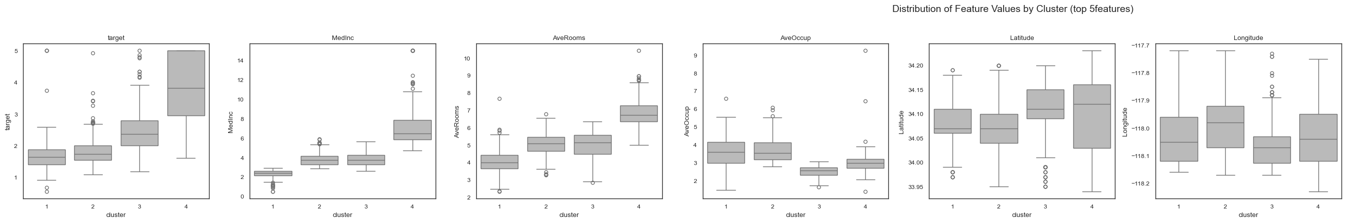
To explore this further, we apply FGC again on the test data, using the same trained Random Forest model. This allows us to assess which of the patterns discovered in the training data persist in the unseen data and which do not.
[6]:
fgc = forest_guided_clustering(
    k=4,
    estimator=rf_housing,
    X=data_housing_test,
    y='MedHouseVal',
    clustering_distance_metric=DistanceRandomForestLCA(),
    clustering_strategy=ClusteringKMedoids(method="fasterpam"),
    JI_discart_value=0.9
)
Using a sample size of 80.00% of the input data for Jaccard Index computation.
Using range k = (4, 4) to optimize k.
Optimizing k: 100%|██████████| 1/1 [00:09<00:00, 9.79s/it]
Clustering Evaluation Summary:
 k   Score  Stable  Mean_JI                               Cluster_JI
 4 0.40895    True    0.971 {1: 0.985, 2: 0.969, 3: 0.943, 4: 0.988}
[7]:
feature_importance = forest_guided_feature_importance(
    X=data_housing_test,
    y='MedHouseVal',
    cluster_labels=fgc.cluster_labels[4],
    feature_importance_distance_metric="wasserstein",
)
plot_forest_guided_decision_paths(
    data_clustering=feature_importance.data_clustering,
    feature_importance_global=feature_importance.feature_importance_global,
    feature_importance_local=feature_importance.feature_importance_local,
    model_type=fgc.model_type,
    num_cols=9,
    draw_heatmap=False,
    draw_distributions=True,
    draw_dotplot=False,
    top_n=5,
)
100%|██████████| 8/8 [00:00<00:00, 1069.57it/s]
🏁 Conclusions#
By comparing the feature-wise distribution plots from the FGC runs on both the training and test sets, we observe both commonalities and differences:
Features like
MedInc,AveRooms, andAveOccupexhibit consistent trends across clusters in both datasets.In contrast, features such as
Latitude,Longitude, andHouseAgeshow weaker or inconsistent trends in the test set, especially for clusters representing intermediate housing values.
These shifts suggest that the model may have learned patterns specific to the training data, particularly those involving geolocation and house age, which do not generalize well. This not only explains the drop in test performance, but also highlights the value of FGC for testing the stability of feature-cluster relationships across datasets.